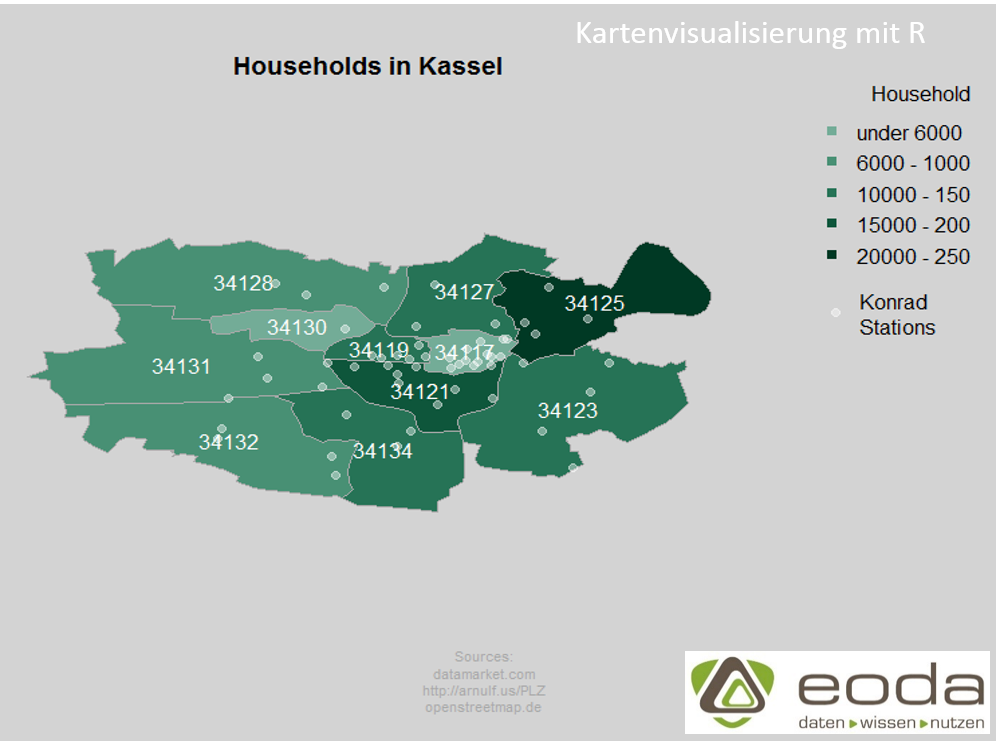
This tutorial shows the creation of a map of the different districts of Kassel including the number of households within each district. This type of map is also known as Choropleth map. Going even further, this map will also contain the stations of the Kassel bicycle sharing system “Konrad”.
Import of shapefiles
The information about map outlines is stored in a Shapefile. Such a Shapefile consists of at least three files.
- A file with the extension shp – it stores the geometric information for the map display
- A file with the extension dbf – it stores the attributes of the geometric figures. In our case, the zip code areas, this file contains the zip codes and the corresponding city names.
- An index file with the extension shx – this enables filtering of geometric data based on corresponding attributes. In our example, we have zip code areas for all of Germany and we only want a subset with the zip codes for Kassel.
In R, a shapefile can be read using the readShapeSpatial command from the maptools package. We get an S4 object of the class Large SpatialPolygonsDataFrame. S4 classes provide a more formal object structure compared to lists and enable more object-oriented work. The object can be indexed like a Dataframe.
shapes <- readShapeSpatial("plz/post_pl.shp")
#subsetting only Kassel shapes
ks_shapes <- shapes[shapes$PLZORT99 == "Kassel",]
Using plot(ks_shapes) the outlines are displayed in R.
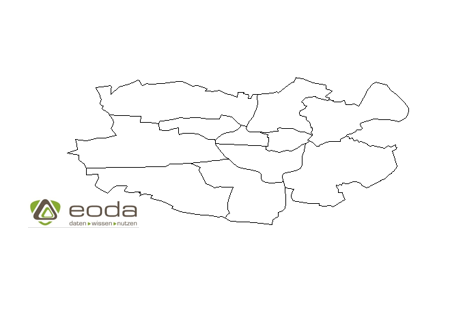
This rudimentary map will now be enriched with further data.
Data Management
The corresponding data comes from the datamarket.com site and was provided by the Kassel statistical office. The data mentioned is specified at the district level, however, the map is based on postal codes. Therefore, another dataset is needed that maps the districts to the corresponding postal code areas. Such an assignment can be found, for example, on Wikipedia.
In R, read in with read.csv2, the data looks like this:
districts_ks <- read.csv2("data/mapping_postalcodes_districts_kassel.csv",
stringsAsFactors = FALSE)
districts_ks
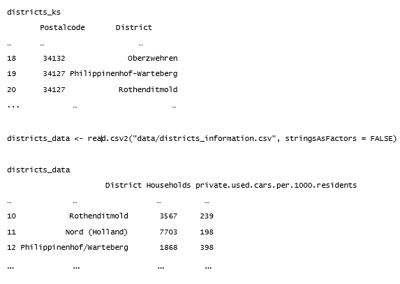
districts_data <- read.csv2(„data/districts_information.csv“, stringsAsFactors = FALSE)

districts_data

District Households private.used.cars.per.1000.residents
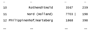
In order to merge the two different datasets, it is necessary to standardize the District variables. For example, one dataset might have the designation "Philippinenhof-Warteberg," while the other has "Philippinenhof/Warteberg." In these small datasets, we simply change the names through indexing and assignment. (For larger datasets, a systematic data cleaning should be performed beforehand. Regular expressions can help with this, allowing text to be searched based on patterns.) <pre>#correction of district names in districts_data districts_data$District[districts_data$District == "Nord (Holland)"] <- "Nord-Holland" districts_data$District[districts_data$District == "Philippinenhof/Warteberg"] <- "Philippinenhof-Warteberg" districts_data$District[districts_data$District == "Süsterfeld/Helleböhn"] <- "Süsterfeld" districts_data$District[districts_data$District == "Wolfsanger/Hasenhecke"] <- "Wolfsanger-Hasenhecke"</pre> The two datasets are then merged using the merge function. <pre>districts_data <- merge(districts_data, districts_ks, all.x = TRUE)</pre> <div></div> <div>We get the following dataset:</div>
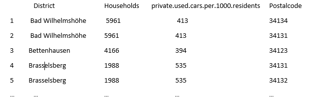
To avoid duplicate entries for District and Postalcode, we will consolidate the data so that we have unique entries for the variable Postalcode. We will sum the values of Households and concatenate the corresponding Districts into a string. For aggregation, we will use the data management package dplyr, which introduces its own grammar for data management. An important component is the Pipe Operator %>%. Originally from the magrittr package, %>% allows chaining function calls without needing to manually reference the dataset each time.
#aggregation by postalcode
data.agg %>% group_by(Postalcode) %>% summarise(
  District = paste(unique(District), collapse = " & "),
  Households = sum(Households),
  cars = sum(private.used.cars.per.1000.residents)
)
The resulting dataset looks as follows:

Postal code areas distributed. For example, how many of the 5040 households in the Mitte district are allocated to the postal code area 34121 and how many to 34117?
To visualize the data on the map, it needs to be divided into classes. Using the `cut` function, we create a factor containing the corresponding classes. In the next command, we assign labels to these classes.
classes <- cut(data.agg$Households[position], c(0,6000,10000,15000,20000,25000))
levels(classes) <- c("under 6000", "6000 – 10000", "10000 – 15000", "15000 – 20000", "20000 – 25000")
We also create a color vector containing five different shades of green.
colours <- c("#73AC97", "#489074", "#267356", "#0E563B", "#003924")
Create Plot
To display the map, we use the graphic functions from Base R. First, we set global parameters of the graphic.
par(mar = c(0,0,1,9), oma = c(3,0,2,1), bg = "lightgrey", xpd = TRUE)
With mar = c(0,0,1,9), we define the inner margins of the graphic. We want no inner margin at the bottom and left, one line at the top, and on the right side should be our legend, for which we define a slightly wider margin of nine lines. With oma = c(3,0,2,1), we define the size of the outer margins. bg = "lightgrey" sets the background of our graphic to light grey. By setting the argument xpd = TRUE, we ensure that the legend is also displayed within the inner frame.
With plot, we finally draw our map, we outline the postal code areas in dark grey and pass as colors our colours vector, sorted by classes (number of households in classes).
plot(ks_shapes, border = "darkgrey", col = colours[classes])
The function text(coordinates(ks_shapes), labels = ks_shapes$PLZ99_N, col = "white") adds labels in the form of postal codes to the areas.
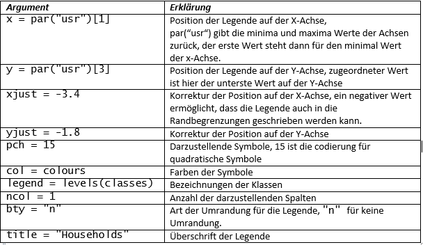
A legend can be added through the function call legend().
legend(x = par("usr")[1], y = par("usr")[3], pch = 15, col = colours, legend = levels(classes), ncol = 1, bty = "n", title = "Households", xjust = -3.4, yjust = -1.8)
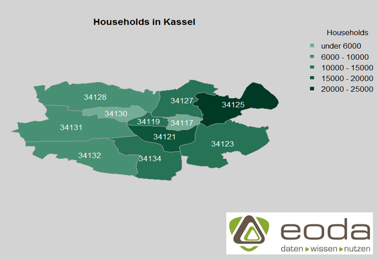
With title("Households in Kassel"), we finally add a title to the graphic.
Integration of information from openstreetmap.de
The information about the coordinates of the stations of the former bicycle rental system Konrad comes from an OSM file that covers the city area of Kassel. You can download such a file from this link. The file itself is structured in XML.
To extract the Konrad coordinates from this file, there are two different possibilities:
parse OSM with the osmar package
The first option uses the osmar package, which is specifically designed for handling OpenStreetMap data. With the commands osmsource_file and get_osm, the file is read and the stored information is placed in an osmar object.
It should be noted that this is done for all information stored for the city area of Kassel and not just for the desired Konrad stations. As a result, the process requires quite a bit of computing power and the resulting object is almost 40MB in size.
If you finally want to access the corresponding nodes of the Konrad stations, you first identify the matching Konrad node IDs with find(OBJ, node(tags(v %agrep% "Konrad"))), then create a corresponding subset of the osmar object that only includes the Konrad nodes with subset(OBJ, node_ids = konrad_id).
Parse OSM with the osmar package
An efficient method for our application is a targeted xpath query. XPath is a query language aimed at extracting information from an XML object. The `xml` package in R provides a functional environment for this purpose.
Using `xmlParse("Kassel.osm")`, the document is read into R. In the next step, we send a query for the latitudes and longitudes respectively and write the result directly into a data.frame.
stations <- data.frame(lat = xpathSApply(osm, path = "//node[tag[@v = 'Konrad']]/@lat"),
lon = xpathSApply(osm, path = "//node[tag[@v = 'Konrad']]/@lon"),
stringsAsFactors = FALSE)
As an argument for `path`, we pass an XPath command that searches for nodes containing a `tag` node with an attribute `v` whose value is "Konrad", and from these nodes, we output the value of the `lat` attribute.

With points(stations$lon, stations$lat, col = adjustcolor("white", 0.4), pch = 19), we add the Konrad stations as white dots to the existing graphic. By using adjustcolor("white", 0.4), we make the white color slightly transparent. We also add another legend element.
legend(par("usr")[1], par("usr")[3], pch = 19, col = adjustcolor("white", 0.4), legend = "Konrad\nStations", bty = "n",
xjust = -5.1, yjust = -4)
And finally, we add a source reference.
mtext("Sources:\ndatamarket.com\nhttp://arnulf.us/PLZ\nopenstreetmap.de", side = 1, line = 1, outer = TRUE, cex = 0.7, col = "darkgrey")
The function mtext stands for margin text and allows text to be written in the margins of a graphic. side = 1 means the text is in the bottom margin, line = 1 denotes text in the second line (the function starts counting at 0), and outer = TRUE indicates that the text should be written in the outer margin. cex and col define the font size and font color, respectively.
The visualization of analysis results and the creation of high-quality, even interactive graphics with R, is one of the topics covered in the eoda Data Science Trainings.
Author
Martin Schneider
Martin Schneider has been working as a Senior Data Scientist and Consultant at eoda GmbH in Kassel since 2012. His main activities are leading data science and AI projects as well as strategic consulting.
Get started now:
We look forward to engaging with you.