Performant, agile and secure: The right infrastructure is the linchpin for the productive use of data science and AI in your company.Professionalize your data infrastructure and create the optimal conditions for your data science workflows – with Posit and eoda.
Get started now: Free Architecture Review Call and 45-day test phase
Book your free Architecture Review Call now with leading infrastructure experts from Posit and eoda and get the target vision and concrete next steps for building your data infrastructure. After that, you will have the opportunity to get to know Posit Workbench, Connect and Package Manager without obligation during a 45-day test phase.
The topics of the Architecture Review at a glance:
Authentication (e.g. LDAP, SAML) and security
Connection to your analysis databases, version control, etc.
Best practices for installing R and Python
Available options for scaling (e.g., Kubernetes or Slurm)
Dealing with package management
Get your IT infrastructure data science-ready now – with Posit’s Professional products.
As one of the Full Service Certified Partners of Posit, we are the contact for Posit interested people and users in Europe. Our services as a Posit partner include consulting, procurement, integration and product trainings.
Let’s evaluate your individual requirements and get the roadmap for your analysis landscape.
Would you like to further push and professionalize data science and AI in your company? The right data infrastructure is increasingly becoming the technical basis for data-centric companies. The central question is how to optimally combine the high development speed and agility of data science and the security requirements of a company infrastructure?
In this online session, learn more about the concrete challenges that data science has posed to companies such as REWE, Covestro or AOK and how they have successfully managed them.
Agenda:
Background: What are the challenges data science brings to existing IT infrastructures?
Realization: How do you identify the pain points in your infrastructure and make it data science-ready?
Added values: What added values are created by implementing a professional data infrastructure?
Learn more about this online session and register now for free.
We are looking forward to your participation! See you soon 😊
In this blog post, we will present 10 Tidyverse functions that are often overlooked by beginners but have proven to be very useful in the right context. We will first describe a problem that we faced in practice in a similar form and then explain how Tidyverse helps us to solve this problem. For the preparation and analysis of data in R, the Tidyverse packages have become an industry standard in the last few years. At eoda, we use many features from the Tidyverse to increase the efficiency of our daily work.
As expected, we start loading the necessary libraries:
library(tidyverse)
1. crossing
Problem:
For the first example, we consider a statistical application. Given two vectors of numerical means and standard deviations, we want to collect all the combination of values that occur in a data frame.
Solution:
The crossing() function from the tidyr package serves exactly this purpose. It takes an arbitrary number of vectors as input and builds all possible combinations of the occurring values:
crossing() can take not only vectors but also data frames as input. In this case all combinations of the rows are formed.
This is especially useful if one of the data frames provides “global” information (in the following example population_data), which is valid for all observations, and the second data frame provides “local” information, which differs between observations or groups (in the example group_data).
As a result of crossing(), we get a single data frame in which each row contains both the global and the group-specific values:
crossing(population_data, group_data)
global_feature_1
global_feature_2
group
local_feature_1
local_feature_2
e
5
1
2
TRUE
e
5
2
5
FALSE
e
5
3
3
FALSE
2. rowwise
Problem:
We stay with the application example from Section 1. For each of the mean-standard deviation combinations, five random values (samples) of a standard normal distribution are to be drawn and added to the data frame in a new column.
Consequently, we need to act at the row level here: Each row of the Data Frame forms a related unit. The newly generated values of the first row are based solely on the remaining values of the first row.
Another peculiarity is that we add multiple entries per cell, not just a single one. In order for this to be compatible with the structure of a data frame, they must be combined into a list. Consequently, the new column is a list column – a column consisting of lists.
Solution:
One way is to use the map()family from the purrr package. The means and standard_deviations columns, to which the rnorm() function is applied, are referenced by the .x and .y placeholders:
For many use cases the rowwise()function from the dplyr package offers a more user-friendly alternative. The column names means and standard_deviations can be used here directly in the call to the rnorm() function without the use of wildcards.
Since the new column consists of lists, the call to rnorm() must be made within list():
When working with ‘list columns‘ the dplyr function nest_by() can be very useful, which unlike tidyr::nest() forms groups line by line.
As an example, we form a separate group for each cyl (cylinder) value from the mtcars dataset. All remaining mtcars columns are bundled into a new column consisting of data frames.
From this, we can add a new column with linear models of mpg (miles per gallon) as a function of hp (horse power).
In a last step, we extract from this the slope coefficients, one number per cylinder value. The result is a single data frame containing the original data, the model objects and the slope coefficients:
From the nested list l, we want to select the string “c” of the lowest level, i.e., the third value of element b in the first list element of a. In total, we have to extract a value from the fourth level of the list.
l <- list(a = list(c(1, 2, list(b = c("a", "b", "c")))))
l
## $a## $a[[1]]## $a[[1]][[1]]## [1] 1## ## $a[[1]][[2]]## [1] 2## ## $a[[1]]$b## [1] "a" "b" "c"
Solution:
This is of course possible without additional packages, but still difficult to read:
l$a[[1]]$b[3]
## [1] "c"
pluck() from the purrr package, on the other hand, solves the task very smartly and easily understandable. The name or index of each level of the list is simply passed sequentially as an argument to the function:
l |> purrr::pluck("a", 1, "b", 3)
## [1] "c"
4. rownames_to_column & rowid_to_column
Problem 1:
The row names of a dataset should be written to the first column. As an example we choose the well known mtcars dataset. In this record the row names describe the model of the car, which should be added to a new model column:
mtcars |> head()
mpg
cyl
disp
hp
drat
wt
qsec
vs
am
gear
carb
Mazda RX4
21.0
6
160
110
3.90
2.620
16.46
0
1
4
4
Mazda RX4 Wag
21.0
6
160
110
3.90
2.875
17.02
0
1
4
4
Datsun 710
22.8
4
108
93
3.85
2.320
18.61
1
1
4
1
Hornet 4 Drive
21.4
6
258
110
3.08
3.215
19.44
1
0
3
1
Hornet Sportabout
18.7
8
360
175
3.15
3.440
17.02
0
0
3
2
Valiant
18.1
6
225
105
2.76
3.460
20.22
1
0
3
1
Solution:
The tibble package provides the function rownames_to_column(). The parameter var can be passed a string with the desired new column name. The new column is automatically placed at the first position of the record.
The second step is to add an index column that uniquely identifies each observation by an ID. To do this, we simply number the rows and write the row numbers in the new column.
Lösung:
An obvious solution creates a new column using mutate() in combination with nrow() or dplyr::row_number() and sets it to the first position using relocate():
Again, the tibble package provides a more condensed solution. rowid_to_column() completes our task in one step. As before, the var argument can be used to specify the name of the new column:
In our daily work with data, we often encounter data sets that need to be cleaned up before they can be reused.
The following data set contains a column with products and another column with associated prices. However, the prices are included in a string without a fixed structure:
The task now is to separate from the strings the numerical prices for each product.
Solution:
A working, but often inconvenient, solution is to use regular expressions. In this example, we look for the first match of at least one digit followed by optional period and decimal places. A disadvantage of this approach is that the result column is still of type character:
However, there is a more comfortable way: The readr package, which is usually used for data import, provides the helper function parse_number(). This scans a vector of strings for the first number and extracts it from its context. Possible decimal places are automatically taken into account.
The new price column in this case belongs directly to the double data type:
In this example, we work with the babynames dataset from the R package of the same name, which lists the most popular baby names in the US over several decades. The column n indicates the absolute frequency of the name within a year:
babynames::babynames |> head()
year
sex
name
n
prop
1880
F
Mary
7065
0.0723836
1880
F
Anna
2604
0.0266790
1880
F
Emma
2003
0.0205215
1880
F
Elizabeth
1939
0.0198658
1880
F
Minnie
1746
0.0178884
1880
F
Margaret
1578
0.0161672
We are interested in what the most frequent letters are for girls’ names to end in the year 2000:
As expected, some letters are in last position much more often than others. For overview purposes, all letters with low frequency should be grouped into a common Other category.
Solution:
The forcats package helps us with this. The fct_lump_*() family aggregates rarer values of a factor (or here character) variable according to various criteria:
fct_lump_n() keeps the n most frequent values and merges all other values into a new category.
fct_lump_min() summarizes all values which occur less often than a given absolute frequency.
fct_lump_prop() summarizes all values which occur less often than a given relative frequency (proportion between 0 and 1).
fct_lump_lowfreq() automatically summarizes the rarest values so that the aggregated Other category still has the lowest frequency among the new categories
In our example, we use fct_lump_n() and keep the most common last five letters:
The parameter w (for weight) can optionally specify a column whose values are summed up to determine the frequency. This is useful if, as in the example above, each letter occurs in only one line and the corresponding frequencies have already been calculated. The parameter is not needed if the frequencies have not yet been calculated and each letter would be duplicated n times in the last_letter column.
7. fct_reorder + geom_col
Problem:
Wir bleiben auch für dieses Beispiel bei dem babynames Datensatz und visualisieren die Anzahl der sechs häufigsten Mädchennamen in einem Balkendiagramm mit geom_col():
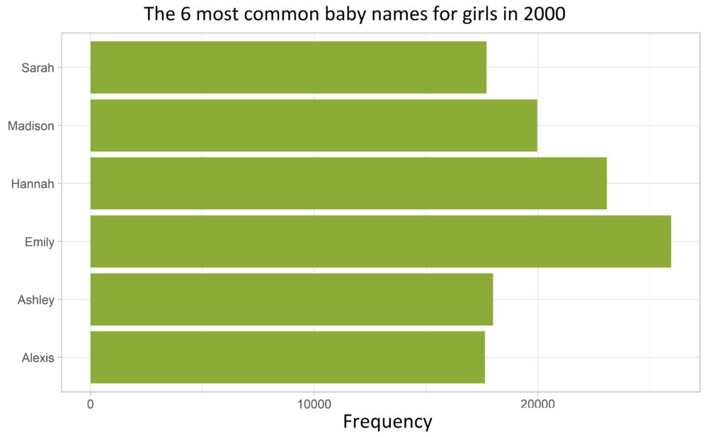
We also stick with the babynames dataset for this example and visualize the number of the six most common girls’ names in a bar chart using geom_col():
plot_color <- "#8bac37"

top_names_females <- names_2000 |>
  filter(sex == "F") |>
  slice_max(n, n = 6)

top_names_females |>
  ggplot(aes(n, name)) +
  geom_col(fill = plot_color) +
  labs(
    title = "Die 6 häufigsten Babynamen für Mädchen im Jahr 2000",
    x = "Häufigkeit", y = NULL,
  ) +
  theme_light() +
  theme(plot.title = element_text(hjust = 0.5))
The names are not ordered along the y-axis according to their frequency!!
Solution:
To achieve this, we reorder the name column according to its frequency (of column n).
This case occurs so often in practice that I use geom_col() almost entirely in combination with fct_reorder() from the forcats package:
top_names_females |>
  mutate(name = fct_reorder(name, n)) |>
  ggplot(aes(n, name)) +
  geom_col(fill = plot_color) +
  labs(
    title = "Die 6 häufigsten Babynamen für Mädchen im Jahr 2000",
    x = "Häufigkeit", y = NULL,
  ) +
  theme_light() +
  theme(plot.title = element_text(hjust = 0.5))
Bonus:
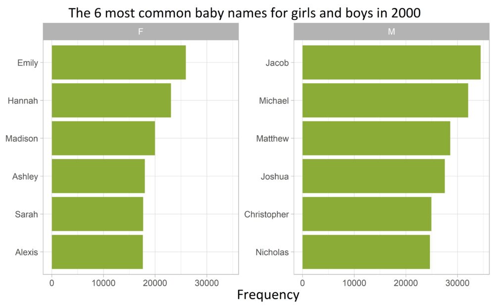
The above procedure no longer works as easily if a separate bar chart is to be plotted in descending frequency for each value of an additional factor variable. As an example, we now additionally consider the most frequent boy names:
top_names <- names_2000 |>
  group_by(sex) |>
  slice_max(n, n = 6)
With fct_reorder(), the bars in each subplot are always ordered according to their frequency in the entire data set (and not just within each value of the sex variable).
The tidytext package, which is primarily used to analyze text data, saves us at this point.
The auxiliary functionsreorder_within()and scale_y_reordered()do exactly the job and sort the values of the factor variables within each subplot:
top_names |>
  mutate(name = tidytext::reorder_within(name, by = n, within = sex)) |>
  ggplot(aes(n, name)) +
  geom_col(fill = plot_color) +
  labs(
    title = "Die 6 häufigsten Babynamen für Mädchen und Jungs im Jahr 2000",
    x = "Häufigkeit", y = NULL,
  ) +
  facet_wrap(facets = vars(sex), scales = "free_y") +
  tidytext::scale_y_reordered() +
  theme_light() +
  theme(plot.title = element_text(hjust = 0.5))
8. separate & separate_rows
Problem 1:
The following dataset should represent the results of different international soccer matches:
However, the game column includes two different types of information: the opponent as well as the result.
Solution:
To make the data frame tidy, we split the game column into two columns using the separate() function from the tidyr package:
data_games |> separate(col = game, into = c("opponent", "result"))
country
opponent
result
Germany
England
win
France
Brazil
loss
Spain
Portugal
tie
Problem 2:
A similar problem occurs when a column contains two pieces of information of the same type in each row. The opponent column now includes only opposing teams, but several per row:
In this case, the desired output does not contain more columns, but more rows, one for each opponent.
Solution:
separate_rows() splits each row of the opponent column into multiple rows, the corresponding country values are duplicated instead:
data_opponents |> separate_rows(opponent)
country
opponent
Germany
England
Germany
Switzerland
France
Brazil
France
Denmark
Spain
Portugal
Spain
Argentina
9. str_flatten_comma
Problem:
A vector of strings is to be combined into a single string. All entries are separated by a comma, only the last two are to be connected by the connecting word “and”.
Without the stringr package, two calls to paste() are required:
First, all entries except the last one are joined by a comma to form a single string.
Then the result from step 1 is concatenated with the last vector entry.
paste(animals[-1], collapse = ", ") |> paste(animals[length(animals)], sep = " and ")
## [1] "dog, mouse, elephant and elephant"
The stringr package provides its own function str_flatten_comma() with the very useful last parameter:
str_flatten_comma(animals, last = " and ")
## [1] "cat, dog, mouse and elephant"
10. arrange + distinct
Problem:
The final example is inspired by work on a recent project of eoda. We have a dataset with two columns, the first column (group) contains an indicator for the group membership of each observation. Within each group, only a single row should be kept: The one with the highest numerical value in the second (value) column:
One possible approach is to use group_by() and slice_max() together:
data_group_value |>
  group_by(group) |>
  slice_max(value, n = 1)
group
value
1
67
2
51
3
79
The disadvantage here is that for large datasets, a large number of groups may be formed, which reduces the efficiency of the calculation. In addition, this approach does not lead to the desired result for duplicates, since slice_max() selects all observations with the maximum value:
data_group_value_duplicates <- data_group_value |>
  mutate(
    value = case_when(
      group == 1 ~ 20L,
      TRUE ~ value
    )
  )

data_group_value_duplicates |>
  group_by(group) |>
  slice_max(value, n = 1)
group
value
1
20
1
20
1
20
1
20
2
51
3
79
So in this case an additional call to slice(1) would be required to really keep only a single row per group.
A more efficient solution resorts to the dplyr combination of arrange() and distinct(). First, all rows within each group are sorted in descending order by their value values. The maximum value to be selected is therefore always at the first position within each group.
In the second step a call to distinct() is sufficient, because this function always keeps the first occurring value in case of duplicates and removes all others from the column
In this article we have illustrated the usefulness of selected Tidyverse functions by means of various examples. Some problems could be solved by other means as well – but only with greater effort
Python, R & Shiny
Our trainings pave the way for your next steps. Machine Learning, Data Visualization, Time Series Analytics or Shiny: Find the right course for your specific needs with us.
Machine Learning, Artificial Intelligence and Big Data – these are the buzzwords you hear every day. But for you they are more than just buzzwords? You are familiar with the methods, technologies and working methods behind them, know how to use them in projects in a target-oriented way and are inspired by the latest developments in the field of data science. You see Data Science as a team discipline, you will work on multifaceted projects, take on responsibility and create added value for leading companies in the DACH region. Look at our job offers Senior Data Scientist, Data Scientist and Project Manager in Data Science – we are looking forward to your application!
For more than 12 years of being a specialist in data science and AI, we not only support our customers with questions about statistics, data analysis and big data, but also our team in its daily development. In a variety of projects, we transform data into added value for leading customers such as OBI, REWE, AOK or Covestro, and with YUNA we develop the platform for the productive use of data science in the company. Creative approaches and innovative technologies: we are shaping the future of digitalization. Join us as a Senior Data Scientist, Data Scientist and/or Project Manager in Data Science.
And that’s not all: we focus on you as an individual! Passion and enthusiasm for our topic, our tasks, and our strong team spirit as well as the opportunity to support our dynamic company development are important to us. Our open corporate culture also offers you a good work-life balance – flexible working times and a free choice of your working place – in our offices in Kassel, Ettlingen, Bochum, Koblenz or from home. Further benefits such as a job ticket, bike leasing, freely selectable vouchers, organic fruit and much more is also available to you. Find out more about eoda and the benefits in our job offerings.
Do’s and Don’ts for the productive use of Shiny applications
When?
20th – 23rd of September 2022, 9 am to 12:30 pm (CET) or
22nd – 25th of November 2022, 9 am to 12:30 pm (CET)
Where?
From your home office or office: Our online Shiny training offers you the opportunity to become a Shiny expert in an uncomplicated, flexible and safe way.
Price?
€999,- per person (excluding VAT)
Who is the course for?
The course is for participants with initial programming experience in R.
What do we offer?
High focus on practice through experienced trainers and application-oriented exercises
High-quality course materials and standardized exercise data sets
Training in small groups for optimal, individual support
Review of learning objectives
Certificate of attendance
Use this opportunity to become a shiny expert with the help of our experienced and certified trainers. Register now!
Our Shiny trainings return! In September and November 2022 our certified instructors teach you how to make your data come to life. As a Full Service Partner of RStudio and leading Shiny expert, we empower you to independently develop successful Shiny apps for productive use in our German-speaking online trainings.
What is covered in the course?
Introduction to Shiny
Philosophy of Shiny: Reactive Programming
Data structures and their properties
User Interface Design
Workflow for developing a Shiny application
Extension packages around Shiny
Do’s and Don’ts for the productive use of Shiny applications
When?
20th – 23rd of September 2022, 9 am to 12:30 pm (CET) or
22nd – 25th of November 2022, 9 am to 12:30 pm (CET)
Where?
From your home office or office: Our online Shiny training offers you the opportunity to become a Shiny expert in an uncomplicated, flexible and safe way.
Price?
€999,- per person (excluding VAT)
Who is the course for?
The course is for participants with initial programming experience in R.
What do we offer?
Our trainers design these courses to be highly practice oriented. They contain application-oriented exercises, which are based on uniform exercise data sets, and high-quality course materials. Trainings are limited to small groups for optimal, individual support. All participants will receive a certificate of attendance.
Use this opportunity to become a shiny expert with the help of our experienced trainers. Register now!
With strong problem-solving skills and focused on the requirements of our customers, you will work on varied projects as part of an interdisciplinary, agile team. You develop existing systems, integrate new ones and check the individual components with regard to performance and usability in times of data-driven business processes. Check out your specific tasks and profile requirements here.
Consulting, implementation, support – for more than 10 years, we have been finding long-term solutions for established companies with the help of our in-depth knowledge of the diverse data science toolset of our eoda | analytic infrastructure consulting. In a variety of projects, we transform data into added value for leading customers such as REWE, University of Amsterdam or Covestro, and with YUNA we develop the platform for the productive use of data science in the company. Creative approaches and innovative technologies: We are shaping the future of digitalization. Dive into the most exciting industry of the 21st century.
And that’s not all: We focus on you as an individual! Passion and enthusiasm for our topic, our tasks and our strong team spirit as well as the opportunity to support our dynamic company development are important to us. Further benefits such as a job ticket, bike leasing, freely selectable vouchers, organic fruit and more.
Our open corporate culture also offers you a good work-life balance – flexible working hours and a freely choosable work location – in our offices in several cities in Germany or from home. A full job description and application form can be found here.
Become part of us now. We are looking forward to your application!
Tell your data story – interactive and understandable with Shiny.
As a Full Service Partner of RStudio and leading Shiny expert, our certified Shiny instructors enable you to independently develop successful Shiny applications for productive use – in our German-speaking online training.
You are already familiar with writing code in R, know the most widely used packages and have already built Shiny apps? As the number of Shiny applications in an organization, the number of developers and the complexity of the application itself increases, it becomes more important to have a framework of best practices to guide the development process. Our guide includes a brief introduction into a possible project management framework, first actions when starting a new project and a technical section for the development process. Download now.
As one of the Full Service Certified Partners of RStudio, we are the contact for RStudio interested people and users in Europe. In addition to our exclusive services, you also benefit from further advantages around the leading RStudio solutions until the end of the year.
We support you from consulting, purchasing (in €) and integration to the operation of RStudio Professional products in your company. Even more: With our R trainings and individual workshops, we enable you to use the R packages and products developed by RStudio in an efficient way.
Our services for your company
Consulting: RStudio Teams, RStudio Workbench, RStudio Connect or RStudio Package Manager? Are you interested in one of RStudio’s solutions? Together with you we evaluate the applications about your individual requirements and find the right solution for your analysis landscape.
Procurement: As a sales partner we can offer you the products of RStudio in Euro. With us, you benefit from a German contractual partner and simplified processes for your purchasing. Beyond the optimal handling of procurement, we keep an eye on the contract terms of your RStudio components and inform you proactively when an extension is necessary.
Integration: As an RStudio integration partner, we implement a seamless integration of the RStudio products for you and help you get started technically. In addition, we share our expertise in using the RStudio products to help you achieve a quick sense of accomplishment. In addition, we are at your side with technical support.
Training: With our R trainings and individual workshops we put you in the position to use the R packages developed by RStudio optimally for yourself.
Get exclusive insights and benefit from advantages now – with eoda.