Whether „Driving Home for Christmas“, „Winter Wonderland“, „Let it snow!“ or „Last Christmas“ – every year christmas songs are taking over the charts again. While average Joe is joyfully putting on the next christmas song, the data scientist starts his journey of discovery through the snowy music history.

 

The data set comes from 55000+ Song Lyrics, which contains over 55,000+ songs. It is a data frame with 55,000+ rows and four columns:

• artist
• song
• link
• text

Our goal is to perform a comprehensive analysis of the song texts to identify the Christmas songs. In order to do so, first we add an additional column to the data frame to give each song a label of either Christmas or Not Christmas, where every song which contains the words Christmas, Xmas or X-mas will be labeled as Christmas and otherwise as Not Christmas.
This is just the initialization of the labels, later we will apply Naive Bayes to a training set to identify the other Christmas songs. First of all, we will start by exploring the data set by means of some intuitive descriptive approaches.
We should start with the data cleaning and tokenization. Afterwards, the Christmas songs will be selected and saved as a variable.
Now we can start analyzing the initial Christmas songs by means of correlations from different perspectives. In the following, we will visualize the correlations with the networkD3 html widget where nodes with the same total number of connections will be given the same color and the color of the edge implies the number of common neighbors shared by two nodes. Moreover, the size of a node indicates the centrality of it, which is defined by the betweenness, i.e. the number of shortest paths going through it. Where the distance between two nodes is the minimum maximum transformation of 1 minus the correlation, which makes sense because intuitively the higher the correlation, the nearer two nodes should be. Moreover, the shorter the distance, the wider the edge.

Note that the correlations are always based on lyrics.

The correlation between words which appeared more than 100 times and are correlated with at least one other word with a correlation greater than 0.55.

The correlation between songs which are correlated with at least 3 other songs with a correlation greater than 0.75. With this, we may detect similiar or just slightly modified songs.

The correlation between certain words

The correlation between artists

Word cloud of the initial Christmas songs

Naive Bayes is a popular supervised machine learning algorithm to handle classification problems with a huge amount of features. It is „naive“ in the sense that, conditioned on a class, the features are assumed to be independently distributed. In our case, we would like to know, given a bunch of features, i.e. the tf-idf of words in a document, whether a song should be classified as Christmas song or not by Naive Bayes.

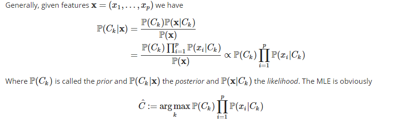
The harder part of constructing the maximum likelihood estimator is the choice of the prior distribution, i.e. the probability distribution of the classes. Where it is usually assumed to be uniformly distributed or estimated by the class frequencies. In our case the multinomial distribution for the likelihood and the uniform distribution for the prior are used, which means we have no prejudice regarding the categorization of the songs without given further information.

So we have identified 2965 hidden Christmas songs and there are 2 songs out of the initial 500 Christmas songs that are rejected by Naive Bayes as Christmas songs.

Explore the hidden Christmas songs

We have therefore successfully identified a bunch of religous christmas songs, whose titles usually do not contain the word „Christmas“ or „X-mas“.

Latent Dirichtlet Allocation & t-Statistics Stochastic Neighbor Embedding

Data Preparation

Only the top 300 features for the Christmas songs including the hidden ones will be used to calculate the Rtsne & LDA, else the memory space will not be sufficient.

LDA

LDA stands for Latent Dirichtlet Allocation, which was introduced in Blei, Ng, Jordan (2003). It is a generative probabilistic model of a corpus, where the documents are represented as random mixtures over latent topics and for a single document there are usually only a few topics that are assigned unneglectable probabilities. Moreover, each topic is characterized by a distribution over words, where usually only a small set of words will be assigned significant probabilities for a certain topic. Either the variational expectation maximization algorithm or Gibbs sampling is used for the statistical inference of the parameters.

LDA requires a fixed number of topics, i.e. it assumes that the number of topics should already be known before applying the algorithm. However, there are possibilities to determine the optimal number of topics by different performance metrics, see Nikita, by using the package ldatuning.

Therefore, we will choose 8 as the optimal number of topics.

We may use the package tidytext to inspect the topic probability distribution of each document, i.e. for each document the sum of the probabilities that it belongs to a topic from 1 to 8 is equal to 1.

Analogously, we can also obtain the probability distribution of words for each topic, i.e. for each topic the sum of probabilities that it generates different words is equal to 1.

The top terms for each topic are:

t-SNE

Developed by van der Maaten and Hinton (2008), t-SNE stands for t-Statistics Stochastic Neighborhood Embedding, which is a dimensionality reduction technique that is formulated to capture the local clustering structure of the original data points. It is non-linear and non-deterministic.

 

The following computation will take about 30 minutes.

What if we repeat the procedure for more than one iteration?

So far we have only run the Naive Bayes for one iteration. However, we may repeat this procedure for more than one iteration, i.e. train a Naive Bayes classifier and relabel all the false positives as Hidden Christmas/Christmas and all the false negatives as Hidden Not Christmas/Not Christmas over and over again.

First of all, we prepare the data again to avoid bugs.

Run 10 iterations.

Then the precision as well as the f1 score grow monotonically at first and then converge to a value around 0.95, which means there are not many „Hidden Christmas Songs“ and „Hidden Not Christmas Songs“ left to be detected. However, in this procedure we always believe that the Naive Bayes classifier is 100% accurate, which is hardly possible. Thus, in each iteration there are some songs falsely classified by Naive Bayes as „Christmas“, which will be used in the next iteration in the training set to train the Naive Bayes classifier. With this accumulating error we might have the apprehension that the results are actually worse with more iterations.

At the end we have roughly half of the songs classified as „Christmas“ and the other half as „Not Christmas“, which seems very implausible. It raises the question whether or not there is an optimal number of iterations, however, we simply can not manually control whether all the 57,650 songs are correctly classified or not. This remains an open question to be answered.

For further information and visualizations please visit us on github and download the notebook.